Introduction

The focus of this project was on Tensor Product B-Spline Patches. The goal was to create a windowed application that would allow a user to model with B-Spline surfaces and then to be able to ray-trace those surfaces with relative speed. In the process of building the application, the hope was to learn about the techniques involved in quickly evaluating and intersecting B-Spline surfaces and, to a lesser extent, learn about some of the challenges in creating a user interface which allows for simple modeling of such surfaces.

Objectives

-Create a windowed application that allows the user to create and modify B-Spline surfaces.

-Allow the loading of B-Spline surface models in the s3d file format.

-Allow the user to ray-trace exactly what is seen in the modeling window.

-Implement a fast evaluation algorithm for B-Spline surfaces.

-Implement both a tessellation scheme and a direct intersection scheme for B-Spline surfaces.

-Implement a procedural bounding box algorithm which subdivides individual surfaces.

-Improve render times by adding multi-threading support to the ray-tracer.

-Compare visual results and time taken to render using tessellation and direct evaluation.

Algorithms

For a fast surface evaluation scheme, I chose to implement Bi-Cubic interpolation, an extension of De Boors algorithm. Given a grid of control points in space and two knot vectors, parameterized by u and v, the algorithm first evaluates each row of points as a B-Spline curve along the u direction. Then these evaluated points are used as control points for the evaluation of a B-Spline curve in the v direction.

Because the partial derivatives at the point of evaluation are needed for Newton Iteration, used for intersection of the surface, the algorithm is modified slightly to obtain them. When first evaluating each row of points, we would normally proceed by interpolating neighbourhood points at each tier of the evaluation tree and continue until only one point remained. Instead, this process is stopped one step short, producing two points. This is done for each row and then, in a similar way, two evaluations in the v direction must occur for our two columns of points and both of these evaluations stop one step short. Finally, this produces 4 points. Taking a difference of points in the u or v directions gives us our partial derivative with respect to u or v respectively. Lastly, the final step for each evaluation can proceed on each direction to give the point of evaluation. The algorithm is advantageous because requires fewer steps than similar algorithms like Bi-linear interpolation and it requires little extra work to produce both partial derivatives. Furthermore, it is more simple to debug than an algorithm like B--Spline Basis Function evaluation because at each step it is clear geometrically what is happening.

To accomplish direct intersection of B-Spline surfaces, I followed [1] and used Newton Iteration. An iterative technique is required here because our B-Spline surfaces may be high degree polynomials, making the prospect for an analytic solution grim. Although Newton Iteration is well known and widely used in the simple 1d case, in the 2d case the details can get tricky. The basic idea is to generate a good initial guess of where a ray will intersect the surface and then to use the partial derivatives of the surface at that point to move closer to the actual point of intersection in the next step. Because Newton Iteration is really a root finding method, the ray is represented as two perpendicular intersecting planes and our system solves for the distance from the planes to the estimate at each step. The root of the system is where the estimate, which lies on the surface, lies on both planes as well. An important parameter in this algorithm is the error bound which deems the estimate close enough to the actual point of intersection. When made too small, our algorithm recurses for longer than is needed wasting CPU time. When made too large, visual artifacts are produced. These arise from sampling normal and colour data from the wrong place on the surface and from the ray-tracer encountering difficulties performing correct lighting calculations. Some effects of these kinds can be seen in the comparison.

To get a good initial estimate for Newton Iteration, again I followed [1] and used procedurally generated bounding boxes. Some initial estimate will not converge if they are too far from the actual point and in general it is dependent on how flat or bumpy the surface is. My algorithm begins dividing the entire u,v domain into 4 sub-regions and creating a box which encompasses the extents of the surface for each of those sub-regions. If the curvature within any of the sub-regions is too high, this process is applied recursively to that sub-region until a depth bound is met or each region is sufficiently flat. My analysis of the flatness of the region takes the dot product of the normals evaluated at corners of the region diagonal from one another and checks that they are above some value. Specifically, I chose 0.8 as the value for this flatness check and a maximum of 4 sub-divisions of a region. These values seemed to work okay in tame circumstances but as seen below in the comparison, they do not hold up as well under regions of high curvature.

It should be noted that the bounding boxes used were axis aligned with a quick intersection test and that for the purposes of increasing speed of tessellation, the same boxes were used to break up the regions of the mesh when tessellating. After seeing the results and further thought, the latter practice is clearly questionable. If more time were available, a spatial subdivision algorithm or at least a completely different bounding box scheme would be a much better choice for this application.

Results and Comparison

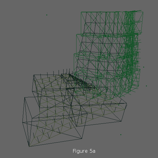
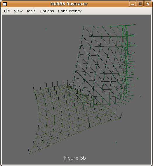
Here we compare visual results and render time of the standard B-Spline Basis function evaluation method to the Bi-Cubic evaluation scheme and tessellation versus direct evaluation. To do so, I created a simple abstract scene with two cubic B-Spline patches and gave them some reasonably interesting curvature to test on. Figure 5b shows the scene as it appeared in the modeling window and figure 5a shows the bounding boxes that were generated in the scene. Two areas of interest are the far right where the vertical surface has a tight bend and the region at the back of the horizontal surface where it was given a tight fold. Note that all renders were done using 16 threads on an Intel Core 2 Quad processor.

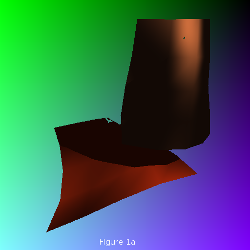
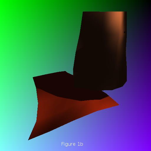
In the first comparison, surfaces were evaluated with a low level of tessellation. Figure 1a shows the scene rendered using the basis function evaluation, figure 1b shows the scene rendered using the Bi-Cubic method. Both scenes took 8 seconds to render. This is because the time spent evaluating the small number of polygons was insignificant compared to the time spent rendering the tessellated surface. Clearly the image in Figure 1a suffers from the overcrowding of bounding boxes in horizontal surface, again giving reason to use with a different scheme for dividing a tessellated region. Surprisingly, the Bi-Cubic evaluation seems to have held up better to these conditions, almost certainly because of better numerical stability properties.

The second comparison shows the surfaces evaluated with a higher level of tessellation. In in this case the Bi-Cubic method (Figure 2b) was slightly faster, taking 15 seconds as opposed to 16 seconds for the basis function method, due to the increased number for evaluations. Again the Bi-Cubic method seems to produce a slightly better image quality.

The third comparison shows the surfaces rendered using the direct intersection technique. Because evaluation occurs for each pixel on screen, the Bi-Cubic method (Figure 3b) was dramatically faster at 13 seconds versus 34 seconds to render Figure 3a using the B-Spline basis functions. Once again, in all the trouble regions, the Bi-Cubic method seems to have produced a better result although both methods seemed to do poorly in the region where the light is at a wide angle to the surface. In general, this seems to be a difficulty experienced in the direct evaluation technique and these areas seem to require much higher accuracy to produce decent visual quality. One curiosity is the relative brightness of these two renders versus those made using tessellation as all normals were normalized. It must be some quirk in the mesh intersection code although nothing obvious sticks out.

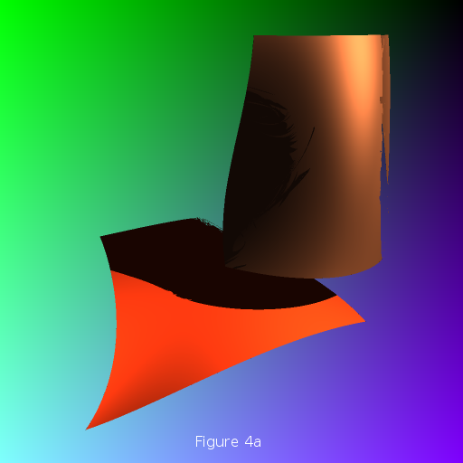
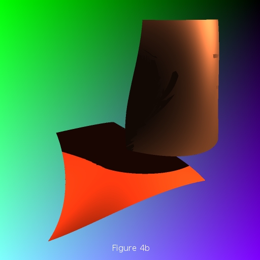
The final comparison was just done to verify the relative time difference between the Bi-Cubic method and the basis function method. Again the scene was rendered using direct evaluation but this time with super-sampling so that each pixel is composed of the result of 4 rays. Figure 4a, using the basis function evaluation took 131 seconds versus only 47 seconds to evaluate using the Bi-Cubic method.

Conclusions and Next Steps

The tests presented showed that the given implementation of the fast evaluation technique was approximately two and a half times faster than the implementation of standard basis function evaluation technique. Furthermore, it appears to be much more numerically stable. Although there was not sufficient time, it would be interesting to implement the fast version of the basis function technique, presented in [1], and compare which fast evaluation scheme is better in practice.

Implementing the direct intersection algorithm based on Newton Iteration made clear the types of problems encountered using iteration techniques and the difficult in implementing them correctly. However, I was surprised that the scene could be rendered without tessellation in less than double the time of the low detail tessellation scene and less time than the high detail tessellation scheme. Despite the artifacts, even at a distance from the surfaces, the direct intersection technique looks better in many places than even the highly tessellated scene. Furthermore, using direct evaluation, the scene does not lose any detail when zooming in, where as the same can not be said for a pre-tessellated scene. In essence, with a little work on removing the artifacts, the tests performed in this project are a proof of concept for direct intersection of B-Spline surfaces versus tessellation.

Finally, as mentioned above, using the same bounding box scheme for direct intersection and mesh subdivision was a mistake. In order to get a true representation of the possible speed and quality of pre-computing a tessellated surface and then rendering it, a different structure needs to be implemented.

References

1.) Oliver Abert, Markus Geimer, Stefan Muller. Direct and Fast Ray Tracing of NURBS Surfaces, Universitat Koblenz-Landau, Forschungszentrum Julich, Universitat Koblenz-Landau

2.) Ching-Kuang Shene. Derivatives of a B-spline Curve, Michigan Technological University. http://www.cs.mtu.edu/~shene/COURSES/cs3621/NOTES/spline/B-spline/bspline-derv.html

3.) Stephen Mann. A Blossoming Development of Splines, University of Waterloo, 2006.